Introduction to Canonical Deletion

by Derrick Stolee

Today, I discuss McKay’s isomorph-free generation technique, commonly called canonical deletion, or canonical construction path. The technique guarantees that every unlabeled object of a desired property will be visited exactly once. The word visited means that a labeled object in the isomorphism class is generated and tested for the given property and possibly used to extend to other objects. Also, objects that do not satisfy the property are visited at most once because we may be able to use pruning to avoid generating objects that do not lead to solutions.

The canonical deletion technique is so called from its use of reversing the augmentation process in order to guarantee there is exactly one path of augmentations from a base object to every unlabeled object. Essentially, a deletion function is defined that selects a part of the combinatorial object to remove, and this function is invariant up to isomorphism. Then, when augmenting an object this augmentation is compared to the canonical deletion of the resulting object to check if this is the “correct” way to build the larger object. If not, the augmentation is rejected and the larger object is not visited. By following the canonical deletion from any unlabeled object, we can reconstruct the unique sequence of augmentations that leads from a base object to that unlabeled object. Further, this process is entirely local: it depends only on the current object and current position within the search tree. This allows the process to be effective even when parallelizing across computation nodes without needing any communication between nodes, unlike some other isomorph-free generation methods which require keeping a list of previously visited objects. Along the way, we will use a consistent example of generating a certain class of graphs to make the discussion more concrete.

Disclaimer: This post was adapted from a background chapter of my Ph.D. thesis. It was written to provide a different perspective on the very abstract nature of the generation algorithm. There are some very subtle points that can be missed easily in McKay’s original paper.

Objects, Augmentations, and Deletions

Suppose we are searching for combinatorial objects from a family ${\mathcal L}$ of labeled objects. Under the appropriate definition of isomorphism for those objects, let $\cong$ be the isomorphism relation and ${\mathcal U}$ be the family of unlabeled objects: the equivalence classes under $\cong$ . Let $P : {\mathcal L} \to \{0,1\}$ be a property, and we wish to generate all objects $X$ in ${\mathcal L}$ where $P(X) = 1$ . We shall assume the property $P$ is invariant under isomorphism ( $\cong$ ): for all unlabeled objects ${\mathcal X} \in {\mathcal U}$ and labeled objects $X, X' \in {\mathcal X}$ , $P(X) = P(X')$ . In this case, we can define $P({\mathcal X})$ for an unlabeled object ${\mathcal X}$ to be equal to $P(X)$ for any labeled object $X \in {\mathcal X}$ .

Example: Let ${\mathcal L}$ be the set of graphs of order $n$ . Then ${\mathcal U}$ is the family of unlabeled graphs where the standard relation of isomorphism ( $\cong$ ) is used between graphs. The property $P$ could be $P(G) = 1$ if and only if $G$ is 4-regular and $G$ has chromatic number three. One nice aspect of the property $P$ is that all induced subgraphs of 4-regular 3-chromatic graphs have maximum degree at most 4 and chromatic number at most 3.

We require a set $B \subset {\mathcal L}$ of base objects and an augmentation. Let $B \subset {\mathcal L}$ be a set of labeled objects where every pair $X, Y \in B$ has $X \not\cong Y$ .

For a labeled object $X \in {\mathcal L}$ , the augmentation defines a set ${\mathcal A}(X)$ of augmentations. An object in ${\mathcal A}(X)$ should specify enough information to determine how to augment $X$ to create a new object $Y$ . Let ${\mathcal D}(X)$ be the set of deletions, which specify the information to determine how to delete something from $X$ to create a smaller object $Z$ .

There must be a bijection $\delta : \cup_{X \in {\mathcal L}} {\mathcal A}(X) \to \cup_{Y \in {\mathcal L}} {\mathcal D}(Y)$ from augmentations to deletions. In some sense, this bijection should be natural, in that an augmentation $A \in {\mathcal A}(X)$ maps to $\delta(A) = D \in {\mathcal D}(Y)$ if and only if performing the augmentation $A$ on $X$ creates the object $Y$ and performing the deletion $D$ on $Y$ results in $X$ .

We shall consider our objects as being built up, so the set of augmented objects ${\mathcal A}(X)$ can be called the above objects while the deleted objects ${\mathcal D}(X)$ are the downward objects. (The sets ${\mathcal A}(X)$ and ${\mathcal D}(X)$ were originally called lower objects $L(X)$ and upper objects $U(X)$ by McKay. In addition to the problem that the letters ${\mathcal L}$ and ${\mathcal U}$ are already used for labeled and unlabeled objects, the notation for $L(X)$ and $U(X)$ is confusing because McKay never explicitly states which direction is “up”!.) Figure 1 provides a visualization of these sets with respect to a labeled object $X$ .

Figure 1. Augmentations ${\mathcal A}(X)$ and deletions ${\mathcal D}(X)$ .

Example: Suppose we wish to enumerate all connected graphs of order $n$ . One augmentation step is given by adding a vertex and specifying its neighborhood. Since every connected graph contains an edge, we can start from $K_2$ as a base object (so $B = \{ K_2\}$ ).

Every vertex augmentation is given by specifying the neighborhood of the new vertex in the graph, so every augmentation is a pair $(G, S)$ with $S \subseteq V(G)$ . To guarantee connectedness, we can assume that $S \neq \emptyset$ . To delete a vertex, we must only specify the vertex, so we can let pairs $(G, v)$ with $v \in V(G)$ be a deletion leading to the graph $G - v$ . From this, let ${\mathcal A}(G) = \{ (G, S) : S\subseteq V(G), S \neq \emptyset \}$ , and ${\mathcal D}(G) = \{ (G, v) : v \in V(G) \}$ . The natural bijection $\delta$ can be defined as mapping a graph, subset pair $(G,S)$ to the graph, vertex pair $(H,v)$ where the graph $H$ has vertex set $V(G) \cup \{v\}$ and $H$ has edges given by $E(H) = E(G) \cup \{ uv : u \in S\}.$ Figure 2 shows an example graph $G$ of order three with all deletions and augmentations specified. The augmentations have white circles representing the vertices in $S$ while the deletions have red circles representing the vertex $v$ to delete. Further, the deletions, $(G,v) \in {\mathcal D}(G)$ , are connected to the augmentations of the two graphs of order two and the augmentations, $(G,S) \in {\mathcal A}(G)$ , are connected to the deletions of the graphs of order four.

Figure 2. Vertex augmentations ${\mathcal A}(G)$ and deletions ${\mathcal D}(G)$ for a graph $G$ .

These definitions of augmentations and deletions are based on labeled objects. In order to generate at most one labeled representative of every unlabeled object, we must consider what isomorphism means in this context.

Augmentations and Orbits

For isomorphism concerns, we shall assume that for an unlabeled object ${\mathcal X} \in {\mathcal U}$ , any two labeled objects $X, X' \in {\mathcal X}$ have a bijection $\pi_{X,X'} : {\mathcal A}(X) \to {\mathcal A}(X')$ and $\sigma_{X,X'} : {\mathcal D}(X) \to {\mathcal D}(X')$ such that the following statements hold:

For all $Y \in {\mathcal A}(X)$ , the object $W$ such that $\delta(Y) \in {\mathcal D}(W)$ and object $W'$ such that $\delta(\pi_{X,X'}(Y)) \in {\mathcal D}(W')$ are isomorphic ( $W \cong W'$ ).
For all $Z \in {\mathcal D}(X)$ , the object $W$ such that $\delta^{-1}(Z) \in {\mathcal A}(W)$ and the object $W'$ such that $\delta^{-1}(\sigma_{X,X'}(Z)) \in {\mathcal A}(W)$ are isomorphic ( $W \cong W'$ ).

This allows us to define the augmented and deleted objects ${\mathcal A}({\mathcal X})$ and ${\mathcal D}({\mathcal X})$ for unlabeled objects ${\mathcal X} \in {\mathcal U}$ as well.
Example: If two graphs, $G$ and $H$ , are isomorphic via a bijection $\tau : V(G) \to V(H)$ , then an augmentation $(G, S) \in {\mathcal A}(G)$ maps to $(H, S')$ where $S' = \{ \tau(x) : x \in S\}$ . Further, a deletion $(G,v)$ maps directly to $(H, \tau(v))$ . Therefore, any two isomorphic graphs $G$ and $H$ have a bijection $\pi_{G,H} : {\mathcal A}(G) \to {\mathcal A}(H)$ .
Now, we wish to remove isomorphic duplicates, so the most natural first step is to remove duplicate augmentations. That is, if we are augmenting an object $X$ via two augmentations $A, A' \in {\mathcal A}(X)$ , we should make sure that $A$ is not isomorphic to $A'$ or else $\delta(A)$ and $\delta(A')$ will be isomorphic. These types of decisions can be made using the automorphism group of the object $X$ .

Example: When augmenting a graph $G$ by adding a vertex, if there is an automorphism $\sigma : V(G) \to V(G)$ such that $\sigma$ maps a set $S \subseteq V(G)$ to a set $S'$ , then the augmentations $(G,S)$ and $(G,S')$ create isomorphic graphs $H$ and $H'$ . Therefore, we should compute all set orbits and select exactly one representative from each orbit. [Since this calculation seems inefficient when the sets can have arbitrary size (i.e. $\delta(G)$ is not bounded), McKay’s paper has a workaround to avoid duplications without sacrificing efficiency.]

It is an unfortunate fact that these local orbit calculations are not enough to guarantee that we shall not create duplicate objects. There are several reasons, including:

Augmentations that are not in orbit can create isomorphic objects. See Figure 3.a, where two single-vertex neighborhoods are not in orbit but augmenting by either creates the same unlabeled graph. Figure 3.b shows this ambiguity in the reverse direction, where two deletions from different orbits result in the same graph.

Figure 3. Examples of orbit complications.

There may be two internally disjoint sequences of non-isomorphic augmentations which generate the same unlabeled object. Figure 4 shows two different sequences of three vertex augmentations starting from $K_2$ that generate the same unlabeled object. What is most important is that these paths are internally disjoint with respect to unlabeled objects. Thus, no amount of verifying that isomorphic duplicates are avoided at the next level (or some constant number of levels), eventually some objects will be repeated.

Figure 4. Two disjoint augmentations to the same graph.

These concerns demonstrate that a “bottom up” approach to avoiding duplicate graphs is not satisfactory. The canonical deletion technique avoids this issue by reversing the process: it makes sure that every unlabeled graph has a unique sequence of deletions that leads to a base object.

Canonical Labelings

In order to avoid the previously mentioned pitfalls that lead to multiple labeled representatives of an isomorphism class being visited in the search, we must utilize a powerful tool that allows us to compute invariants.

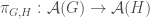
For a family of labeled objects ${\mathcal L}$ whose unlabeled objects are ${\mathcal U}$ , a canonical labeling is a function $\ell : {\mathcal L} \to {\mathcal L}$ where for every unlabeled object $U \in {\mathcal U}$ and every pair of labeled objects $L, L' \in U$ , the two labeled objects $\ell(L)$ and $\ell(L')$ are equal.

In this sense, the labeling function $\ell$ will \textit{relabel} an object $L$ to create another labeled object $\ell(L)$ of the same isomorphism class. The important behavior is that $\ell(L)$ is the same labeled object for the entire isomorphism class, so the object $\ell(L)$ is invariant for unlabeled objects.

Example: When the family of labeled objects ${\mathcal L}$ is a collection of undirected (or directed) graphs, then a canonical labeling $\ell(G)$ can be selected to be the graph $H \cong G$ with lexicographically-least adjacency matrix. This choice of canonical labeling fits the definition, but is difficult to compute. Instead, McKay’s nauty library was designed to efficiently compute canonical labelings. The algorithm defines the map $\ell$ , and is not easily described. See the survey paper by Hartke and Radcliffe for a full description of the nauty algorithm.

Canonical Deletions

Finally, we are able to describe the canonical deletion. This deletion is the most fundamental concern to this search technique. A canonical deletion function is a map ${\mathrm{del}} : {\mathcal L} \to \cup_{X\in {\mathcal L}} {\mathcal D}(X)$ such that ${\mathrm{del}}(X) \in {\mathcal D}(X)$ and for any two isomorphic objects $X \cong X'$ we have isomorphism of their deletions: ${\mathrm{del}}(X) \cong {\mathrm{del}}(X')$ .

Example: When building graphs by vertex augmentations, a graph $G$ has deletion set ${\mathcal D}(G) = \{ (G, v) : v \in V(G)\}$ . Thus, we need only select a single vertex up to isomorphism. By computing the canonical labeling $\ell(G)$ , we find an ordering of $V(G)$ that is invariant up to isomorphism. Therefore, let $v \in V(G)$ be the vertex which maps to the smallest-index vertex in $\ell(G)$ when using an isomorphism from $G$ to $\ell(G)$ . Since the isomorphism used above is arbitrary, this only determines the canonical deletion up to vertex orbits, but this is still appropriately invariant under isomorphism.

WARNING: When restricting to connected graphs, we must be sure that the deletion we select leads to a connected graph. Therefore, the canonical deletion should select the smallest-index vertex that is not a cut vertex.

Given access to a canonical deletion, we can now describe the full canonical deletion algorithm.

CanonicalDeletion( $n, X$ )
if Prune( $X$ )
    // There are no solutions “above” this object.
    return
if IsSolution( $X$ )
    // This object is a solution.
    Output $X$
ifOrder( $X$ ) $\geq n$
    // This object is too large to augment.
    return
for all augmentations $A \in {\mathcal A}(X)$ , up to isomorphism
    // Convert the augmentation into a deletion.
     $D \leftarrow \delta(A)$ .
    // Find the labeled object that corresponds to that deletion.
     $Y \leftarrow {\mathcal D}^{-1}(D)$ .
    // Compute that object’s canonical deletion.
     $D' \leftarrow {\mathrm{del}}(Y)$ .
    // Test if the current augmentation corresponds to that canonical deletion.
    if $D \cong D'$
        // Visit the object $Y$ .
        call CanonicalDeletion( $n, Y$ )
return

The reason this algorithm is correct is due to the fact that following the canonical deletions ${\mathrm{del}}(X)$ in reverse allows you to reconstruct the unique sequence of augmentations that correspond to those deletions (just in reverse order).

Given a labeled object $X \in {\mathcal L}$ , the deletion sequence from $X$ is a sequence $X_0$ , $X_1$ , $X_2$ , $\dots$ , $X_k$ of labeled objects such that

The first object $X_0$ is equal to $X$ .
For $i \in \{1,\dots, k\}$ , $\delta^{-1}({\mathrm{del}}(X_{i-1})) \in {\mathcal A}(X_i)$ . That is, the canonical deletion from $X_{i_1}$ corresponds to an augmentation from $X_i$ .
The last object $X_k$ is a base object: $X_k \in B$ .

Thus, the objects that are visited by the CanonicalDeletion algorithm are exactly those with deletion sequences $X_0,X_1,\dots,X_k$ where Prune( $X_i$ ) never holds and $X_k \in B$ . In the call to CanonicalDeletion( $n, X_{i-1}$ ), only the augmentation $A \in {\mathcal A}(X_{i-1})$ that has $\delta(A) \cong {\mathrm{del}}(X_i)$ will succeed in generating $X_i$ , leading to the call CanonicalDeletion( $n, X_{i}$ ). Since we are restricting to a single representative of the augmentation orbits, this leads to exactly one generation of $X_i$ .

It is very important that we make the distinction that for an augmentation $A \in {\mathcal A}(X)$ we have $\delta(A) \cong {\mathrm{del}}(Y)$ for an augmented object $Y$ and not simply that $X$ is isomorphic to the object resulting from performing the deletion ${\mathrm{del}}(Y)$ on $Y$ . This is due to the fact that multiple non-isomorphic deletions may lead to the same unlabeled object. Recall that Figure 3.b gave an example of such an ambiguity.

Figure 5 presents an example of the complicated network that may exist between the augmentations and deletions of combinatorial objects, but that the canonical deletion selects a subtree structure to this network. Specifically, the canonical deletions are presented as thick lines and there is exactly one path from a given object to the base object.

Figure 5. A network of unlabeled objects with augmentations/deletions.

Example: The algorithm GraphCanonicalDeletion is a specific implementation of the canonical deletion algorithm for generating graphs by vertex augmentations. It restricts to graphs with maximum degree four and chromatic number at most three.

GraphCanonicalDeletion( $n, G$ )
if $\Delta(G) \geq 5$ or $\chi(G) \geq 4$
    // There are no solutions with $G$ as an induced subgraph.
    return
if $n(G) \equiv n$ and $\delta(G) \equiv \Delta(G) \equiv 4$ and $\chi(G) \equiv 3$
    // This graph is a solution.
    Output $G$
    return
if $n(G) \geq n$
    // This graph is too big to extend
    return
for all orbits ${\mathcal O}$ of non-empty sets $S \subseteq V(G)$ with $|S| \leq 4$
    Let $S \in {\mathcal O}$ be any representative.
    // Create the augmented graph.
     $H \leftarrow G + v_S$ .
    Compute that object’s canonical deletion.
     $(H,v') \leftarrow {\mathrm{del}}(H)$ .
    // Test if the current augmentation corresponds to that canonical deletion.
    if $v_S$ and $v'$ are in the same $H$ -orbit
        Visit the graph $H$ .
        call GraphCanonicalDeletion( $n, H$ )
return

Efficiency Considerations

Based on my experience in creating specific implementations of the canonical deletion algorithm, I contribute a few suggested methods for writing more efficient software.

Deletion by filtering

Calling nauty is an expensive computation, so it should be avoided whenever possible. However, we cannot exactly compute the canonical deletion without it, but we can sometimes determine that our current augmentation does not correspond to the canonical deletion without using nauty. Therefore, I instead create a method IsCanonical( $H, A$ ), where $H$ is the augmented graph and $A$ is the augmentation I used to create $H$ . Then, the method can return $\mathsf{False}$ at the earliest time that it detects this is NOT the canonical deletion. This process is then helped by a staged selection of canonical deletion:

Start with an easy invariant metric, such as minimum degree of a vertex. This restricts the possible deletions very quickly in most cases.
Define a sequence of more complicated invariant metrics, such as minimizing the sum of the squares of all the neighbor degrees. Such invariants can remove even more choices without being overly costly to compute.
If all previous restrictions on the choice of canonical deletion did not prove that the current augmentation is not canonical, we have two options. We can check if the list of feasible deletions that fit the previous invariants has size exactly one. If so, then we know without a doubt that this deletion is canonical. Otherwise, we need to select a deletion using a canonical labeling and then check if the current augmentation is in orbit with that canonical deletion. Both of these checks can be done using a single call to nauty.

Reduced augmentation count

In the previous suggestion, we restricted the choice of canonical deletion to a simple invariant minimization, such as minimizing the vertex degree. Making such a restriction as part of your canonical deletion can reduce the number of augmentations you attempt, for instance by only augmenting vertices of degree at most $\delta(G) + 1$ .

Pruning in deletion

Again, since calling nauty is probably the most computationally expensive subroutine in this algorithm, it may be useful to check if the augmented graph should be pruned even before finishing the canonical deletion. This may depend on how complicated your Prune( $G$ ) method is, but if Prune( $G$ ) holds, there is no reason to visit that graph and hence no reason to compute a canonical labeling.

Skipping augmentation orbit calculation

For some augmentations, it may be difficult to completely compute the orbits of augmentations. Vertex augmentations is such an example, because there are many possible neighborhood sets. It may be more beneficial to ignore the automorphism calculation and instead just attempt every augmentation. For every successful augmentation, store a canonical labeling of the augmented object. Then, the objects generated from the current object are visited if and only if the augmentation corresponds to the canonical deletion and that augmented object is not isomorphic to any previous augmentation. By storing a list of visited objects at a given node, we are using the canonical labelings locally, which can be very efficient. See McKay’s original paper for more details about this strategy.

Experiment with the augmentation step

Depending on what type of objects you are generating, there may be something special about their structure that you can exploit in the augmentation step. Observe that in a triangle-free graph every vertex neighborhood is an independent set. McKay provides an example of generating triangle-free graphs by making the vertex augmentations only use independent sets. More radical experimentation of augmentations will be discussed in later posts.

References

S. G. Hartke and A. Radcliffe. Mckay’s canonical graph labeling algorithm. In Communicating Mathematics, 479, 99–111. American Mathematical Society, 2009.

B. D. McKay. Isomorph-free exhaustive generation. J. Algorithms, 26(2):306–324, 1998.

B. D. McKay. nauty user’s guide (version 2.4). Dept. Computer Science, Austral. Nat. Univ., 2006.

2 Comments to “Introduction to Canonical Deletion”

David Kofoed Wind (@utdiscant) says:

August 14, 2012 at 1:52 am

Great post.

There are some $-signs floating around somewhere, which was not converted to LaTeX, I think you should be able to find them all by just search for “$”.

- derrickstolee says:
  
  August 14, 2012 at 1:59 am
  
  Thanks for the heads-up. I thought I caught them all, but I’ll be sure to check more carefully next time.

Computational Combinatorics